 |
|
It is very exciting that the second generation of Iridium satellites, Iridium NEXT (https://www.iridiumnext.com), are in the process of being launched. The first launch of ten NEXT satellites was on 14 January 2017 and the 41st through 50th NEXT satellites were launched on 29 March 2018. That means that 2/3 of the new constellation is already in place, and the new satellites are all performing well!
The Iridium NEXT satellites promise even better input data for AMPERE. In the short term, we are working to ingest and perform the initial processing and calibration of NEXT data. If you thought that in-flight calibration of four space magnetometers was hard (e.g., Cluster and MMS), imagine handling a total of 75! So please bear with us as we work to make this exciting new dataset as high quality as possible.
Beginning in January 2017, you may notice more `gray' satellites in the browser and summary graphics, indicating a lack of data from the original constellation (Block 1). This reflects the replacement within the constellation of Block 1 satellites with NEXT satellites, which we are not yet including in our processing. This leads to a gradual degradation of the data products so that data from January 2017 through September 2017 should be used with caution. The user should pay particular attention to whether the time or region of interest are mostly actual data or delayed data (plotted in gray). Because the AMPERE inversions require a minimum spatial coverage (roughly half of the satellites in each orbit plane, at the least), we have had to pause the spherical harmonic inversions and derived product generation as of 20 September 2017 as we work to integrate the NEXT data (19 September 2017 is the most recent day processed).
When we have our processing of the NEXT data in place, we will re-process all of the AMPERE products from January 2017 forward so these data WILL be available - things are just under construction for a bit longer.
If you have any questions, don't hesitate to contact us. We're always glad to help.
This describes products generated from AMPERE data designed for general release.
All of these products are based on magnetic field data provided under AMPERE. The data being released consist of magnetic field data that has been processed to adjust for satellite attitude to rotate into geophysical coordinates, subtract the Earth’s main field, apply long period de-trending, and transform the residuals and satellite positions into Altitude Adjusted Corrected Geomagnetic (AACGM) coordinates.
The spherical harmonic fit is implemented over the entire sphere of the Earth from pole to pole with a latitude order of 60 (corresponding to a latitude resolution of 3°) and a longitude order of 5 commensurate with the orbit spacing. The spherical harmonic fit is done in Earth centered inertial (ECI) coordinates for two reasons. First, the orbits are nearly fixed in inertial coordinates so that data spliced together from different satellites along a given orbit plane form a continuous track of data. Second, this coordinate system preserves physical dimensions so that derivation of current densities is straightforward. Note that AACGM coordinates do not preserve physical dimensions or orthogonality of vectors so this system cannot be used for this calculation.
To transform vectors from ECI into AACGM the following procedure is used. The North unit vector in AACGM is transformed into ECI and this direction is then dotted with the horizontal vector to yield the ‘true’ north AACGM vector component. The same procedure is used for AACGM East. It turns out that some data are subject to uncertainties that make them unsuitable for use in the AMPERE inversions. Rather than introduce longitude and latitude gaps in the inversion which would obscure the results for the valid data, the unusable data are replaced with interpolated values at the times and positions of the measured data that are not used. The interpolation is between the satellite ahead and behind the satellite whose data are not used. Interpolated data are flagged in digital and graphical data products.
These plots display the input data, reduced magnetic perturbations, spherical harmonic fit to the magnetic perturbation data, and the radial current density. All quantities are shown in Altitude Adjusted Corrected Geomagnetic Coordinates (AACGM). Each plot shows a ten-minute frame of data and the corresponding spherical harmonic fit and radial currents derived as the curl of the spherical harmonic magnetic perturbation fit. Type 1 summary plots show latitudes from 40° magnetic latitude (MLAT) to the pole to ensure coverage throughout strong storms. Type 2 summary plots show latitudes from 60° MLAT to the pole to better resolve the data under typical activity levels. Plots are made for both northern and southern hemispheres.
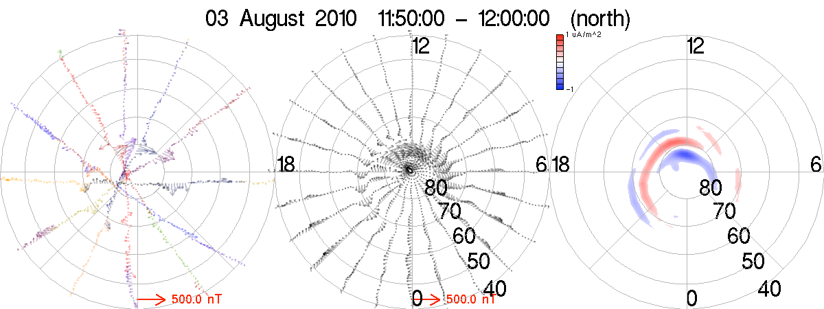
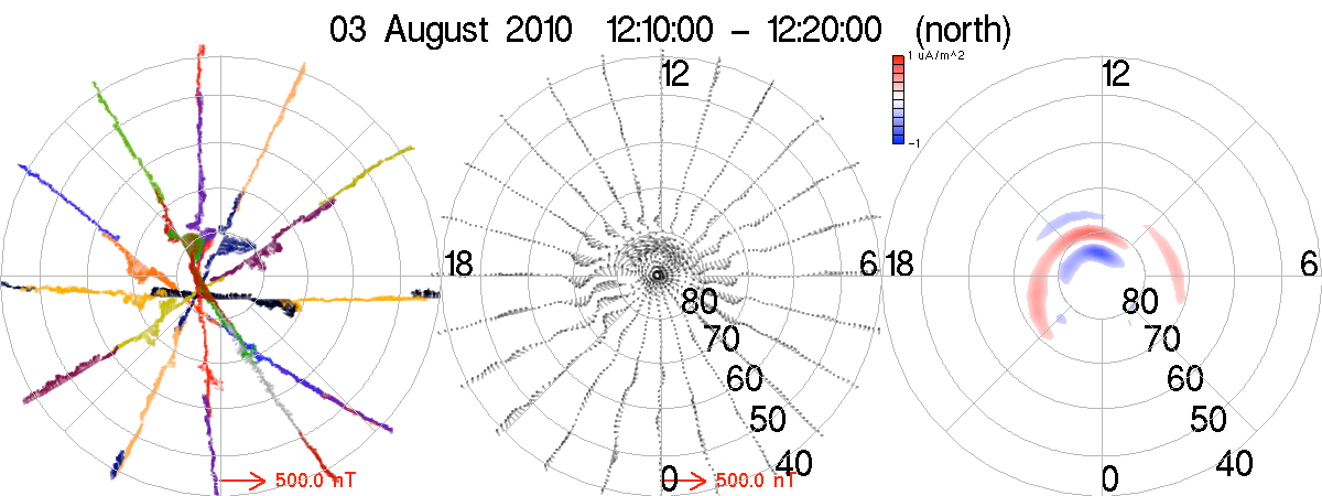
Figure 1. Type 1 summary plots for 3 August 11:50-12:00 UT in standard AMPERE sampling operations and for 12:10-12:20 UT just
following a transition to high-rate AMPERE operations at 12:00 UT. The transparency level of the vectors in the left panel was chosen
to allow overlapping vectors to be seen in high-rate data while still being dark enough to see in low rate data.
Figure 1 shows Type 1 summary plots from 3 August 2010. From left to right these plots show: reduced magnetic field residual data showing the horizontal plane vectors (left); spherical harmonic fit to the magnetic perturbations (center); radial current (right). In the perturbation data plot different colors are used to show measured magnetic field residuals from different satellites’ data. The arrows show the magnetic perturbation using the reference arrow at the bottom of the panel. The tail of each arrow shows the satellite location at the measurement point. The arrows represent the horizontal magnetic perturbation vectors. Grey is used to show interpolated data whereas colors indicate valid data. The arrows are partially transparent to reduce tracks from obscuring other tracks near the orbit crossing zone and when the perturbations are large.
The middle panel shows the horizontal vector from the spherical harmonic fit evaluated with 1 hour longitude by 1° latitude resolution. The black vectors are semi-transparent to make it easier to follow the results through intervals of intense activity and use the same vector scaling as the left-hand data panel.
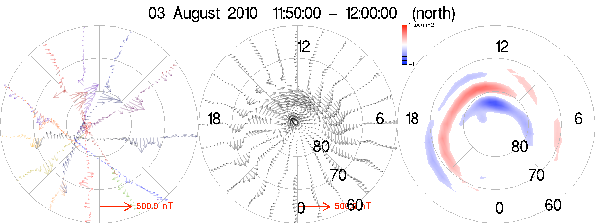
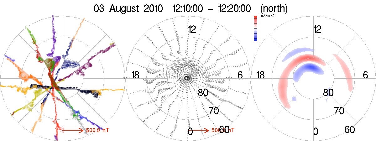
Figure 2. Type 2 summary plots for 3 August 11:50-12:00 UT in standard AMPERE sampling operations
and for 12:10-12:20 UT just following a transition to high-rate AMPERE operations at 12:00 UT.
The right-hand panel shows the radial current density evaluated in inertial coordinates. The positions are translated into the AACGM system. Upward currents are shown in red and downward currents in blue. Current densities with magnitudes below 0.2 m-A/m2 are not shown because these are approximately below the noise level in the data as presently processed.
Figure 1 shows examples of these plots for 03 August 2010 from 11:50-12:00 UT and 12:10-12:20 UT. The first interval shows standard AMPERE data sampling of 19.44 s between samples and the second interval shows high-rate AMPERE data with sampling of 2.16 s between samples. The transition between standard and high-rate was scheduled at 12:00 UT and the order of magnitude in sampling density is evident. At present, AMPERE spherical harmonic fitting does not implement latitude orders corresponding to the higher sampling rate. Plots are generated at 2-minute intervals.
For each type of summary plot movie files (.mov format) are also provided that include all of the frames for each day. A small fraction of the 10-minute frames do not yet process completely for reasons that we have not yet identified. The frames for these intervals do not appear in the movies so that there are occasional jumps of more than two minutes between frames.
A data browser is available that provides custom view of the spherical harmonic fit and radial current density data products. This tool presently provides scalar color-scale image plotting of the fit perturbation magnitude, Eastward component of the fit perturbation, and the radial current density. It does not yet include vector plots of the fit result or of the input data though these are on our list of products to implement in the future.
This browse tool uses a GUI interface to allow variable color bar scaling, lower value clipping, and adjustable latitude range. Various ways of viewing the Earth are available as is an option to show the solar terminator. The tool requires a user registration which is solely used to track users to understand who uses the data and provide a means to allow users to communicate problems they encounter with the browse tool or data products. The browse tool also has a field to report problems.
The processed data products, spherical harmonic fit for the horizontal magnetic field and the radial current density are also provided in daily netCDF files via the data browse tool. These data consist of the horizontal vector magnetic perturbation fits and radial current densities on a regular 1° x 1° latitude longitude grid in Altitude Adjusted Corrected Geomagnetic Coordinates.